Sine and Rotatory Position Encoding

Position Encoding是Transformer重要组成部分，输入序列通过加入对输入位置编码后的信息，使模型有能力分辨不同位置的能力，主要有绝对位置编码和相对位置编码。本文是对苏神的Transformer升级之路系列¹²的个人笔记以及RoPE编码³的学习。

深入三角函数位置编码

位置编码在Transformer原文中的戏份并不多，主要目的是由于自注意力attention的操作是不区分位置的，因此我们需要让模型知道，例如这是第几个词（绝对位置），这个词和另一个词的距离（相对位置）。

虽然知道三角函数位置编码的具体公式和代码，但是很多细节和设计理由并没有深究，比较简单的两个问题是：

位置编码是如何给输入Embedding序列注入位置信息的？
为什么使用相加赋予输入Embedding序列位置信息？

位置编码性质

回顾一下三角函数位置编码：

\begin{equation}\left\{\begin{aligned}\boldsymbol{p}_{k,2i}&=\sin\Big(k/10000^{2i/d}\Big)\\ \boldsymbol{p}_{k, 2i+1}&=\cos\Big(k/10000^{2i/d}\Big) \end{aligned}\right.\end{equation}

其中， $p_{k,2i},p_{k,2i+1}$ 分别是序列中位置 $k$ 处的、在embed_dim上的 $2i,2i+1$ 的位置， $d$ 是embed_dim的大小。

换一种形式可以看到，每个对序列 $k$ 位置的位置编码向量 $\boldsymbol{p}_{k}$ 每个值在奇偶位是 $\sin$ 和 $\cos$ 交替变换:

\begin{equation} \boldsymbol{p}_{k} = \begin{bmatrix} \sin({\omega_0} \cdot k)\\ \cos({\omega_0} \cdot k)\\ \\ \sin({\omega_1} \cdot k)\\ \cos({\omega_1} \cdot k)\\ \\ \vdots\\ \\ \sin({\omega_{\frac{d}{2}-1}} \cdot k)\\ \cos({\omega_{\frac{d}{2}-1}} \cdot k) \end{bmatrix} \end{equation}

其中， $\omega_i = \frac{1}{10000^{2i / d}}$ ，请记住这里奇数和偶数位分别是频率相同的 $\sin$ 和 $\cos$ 组成的一对，后面的RoPE会使用这一个二维向量举例。

为什么上式赋予了Embedding位置信息？

我们先回到问题的原点，如果想要给某个序列添加位置信息，这个位置信息是什么样子的呢？有一些选项：

例如 $[0,1]$ 区间分别代表序列中第一个位置和最后一个位置，但是缺点是如果序列长度变化，不能保证，每个绝对位置上的值不变
或者，可以把位置这个数字直接给到序列，即 $1,2,...,n$ ，但是缺点是序列的位置会变得很大，如果序列非常长的话

总结起来，给序列提供位置信息需要的性质：

每个序列位置的位置编码应该是唯一的
必须是确定性的，是序列位置 $k$ 的确定性函数，不能对不同的序列长度，位置编码是不同的

很多文章使用二进制的数字来表示整型的位置⁴举例对三角函数编码交替进行比较，例如:

\begin{align} 0: \ \ \ \ \color{orange}{\texttt{0}} \ \ \color{green}{\texttt{0}} \ \ \color{blue}{\texttt{0}} \ \ \color{red}{\texttt{0}} & & 8: \ \ \ \ \color{orange}{\texttt{1}} \ \ \color{green}{\texttt{0}} \ \ \color{blue}{\texttt{0}} \ \ \color{red}{\texttt{0}} \\ 1: \ \ \ \ \color{orange}{\texttt{0}} \ \ \color{green}{\texttt{0}} \ \ \color{blue}{\texttt{0}} \ \ \color{red}{\texttt{1}} & & 9: \ \ \ \ \color{orange}{\texttt{1}} \ \ \color{green}{\texttt{0}} \ \ \color{blue}{\texttt{0}} \ \ \color{red}{\texttt{1}} \\ 2: \ \ \ \ \color{orange}{\texttt{0}} \ \ \color{green}{\texttt{0}} \ \ \color{blue}{\texttt{1}} \ \ \color{red}{\texttt{0}} & & 10: \ \ \ \ \color{orange}{\texttt{1}} \ \ \color{green}{\texttt{0}} \ \ \color{blue}{\texttt{1}} \ \ \color{red}{\texttt{0}} \\ 3: \ \ \ \ \color{orange}{\texttt{0}} \ \ \color{green}{\texttt{0}} \ \ \color{blue}{\texttt{1}} \ \ \color{red}{\texttt{1}} & & 11: \ \ \ \ \color{orange}{\texttt{1}} \ \ \color{green}{\texttt{0}} \ \ \color{blue}{\texttt{1}} \ \ \color{red}{\texttt{1}} \\ 4: \ \ \ \ \color{orange}{\texttt{0}} \ \ \color{green}{\texttt{1}} \ \ \color{blue}{\texttt{0}} \ \ \color{red}{\texttt{0}} & & 12: \ \ \ \ \color{orange}{\texttt{1}} \ \ \color{green}{\texttt{1}} \ \ \color{blue}{\texttt{0}} \ \ \color{red}{\texttt{0}} \\ 5: \ \ \ \ \color{orange}{\texttt{0}} \ \ \color{green}{\texttt{1}} \ \ \color{blue}{\texttt{0}} \ \ \color{red}{\texttt{1}} & & 13: \ \ \ \ \color{orange}{\texttt{1}} \ \ \color{green}{\texttt{1}} \ \ \color{blue}{\texttt{0}} \ \ \color{red}{\texttt{1}} \\ 6: \ \ \ \ \color{orange}{\texttt{0}} \ \ \color{green}{\texttt{1}} \ \ \color{blue}{\texttt{1}} \ \ \color{red}{\texttt{0}} & & 14: \ \ \ \ \color{orange}{\texttt{1}} \ \ \color{green}{\texttt{1}} \ \ \color{blue}{\texttt{1}} \ \ \color{red}{\texttt{0}} \\ 7: \ \ \ \ \color{orange}{\texttt{0}} \ \ \color{green}{\texttt{1}} \ \ \color{blue}{\texttt{1}} \ \ \color{red}{\texttt{1}} & & 15: \ \ \ \ \color{orange}{\texttt{1}} \ \ \color{green}{\texttt{1}} \ \ \color{blue}{\texttt{1}} \ \ \color{red}{\texttt{1}} \\ \end{align}

可以观察到：低位(红色)的0和1交替是非常快速的，越往高位走，0和1的交替频率会越低。0和1的交替都是整型，它的浮点数形式就想到了三角函数交替了。

相加

第二个问题：为什么和输入Embedding序列相加？Concat行不行?

tl;dr是其实concat应该也没有太大的问题，但是可能会增加一些参数量。

Reddit上有一个不错的回答[^6]:

In attention, we basically take two word embeddings (x and y), pass one through a Query transformation matrix (Q) and the second through a Key transformation matrix (K), and compare how similar the resulting query and key vectors are by their dot product. So, basically, we want the dot product between Qx and Ky, which we write as:

(Qx)‘(Ky) = x’ (Q’Ky). So equivalently we just need to learn one joint Query-Key transformation (Q’K) that transform the secondary inputs y into a new space in which we can compare x.

By adding positional encodings e and f to x and y, respectively, we essentially change the dot product to

(Q(x+e))’ (K(y+f)) = (Qx+Qe)’ (Ky+Kf) = (Qx)’ Ky + (Qx)’ Kf + (Qe)’ Ky + (Qe)’ Kf = x’ (Q’Ky) + x’ (Q’Kf) + e’ (Q’Ky) + e’ (Q’K f), where in addition to the original x’ (Q’Ky) term, which asks the question “how much attention should we pay to word x given word y”, we also have x’ (Q’Kf) + e’ (Q’Ky) + e’ (Q’K f), which ask the additional questions, “how much attention should we pay to word x given the position f of word y”, “how much attention should we pay to y given the position e of word x”, and “how much attention should we pay to the position e of word x given the position f of word y”.

Essentially, the learned transformation matrix Q’K with positional encodings has to do all four of these tasks simultaneously. This is the part that may appear inefficient, since intuitively, there should be a trade-off in the ability of Q’K to do four tasks simultaneously and well.

HOWEVER, MY GUESS is that there isn’t actually a trade-off when we force Q’K to do all four of these tasks, because of some approximate orthogonality condition that is satisfied of in high dimensions. The intuition for this is that randomly chosen vectors in high dimensions are almost always approximately orthogonal. There’s no reason to think that the word vectors and position encoding vectors are related in any way. If the word embeddings form a smaller dimensional subspace and the positional encodings form another smaller dimensional subspace, then perhaps the two subspaces themselves are approximately orthogonal, so presumably these subspaces can be transformed approx. independently through the same learned Q’K transformation (since they basically exist on different axes in high dimensional space). I don’t know if this is true, but it seems intuitively possible.

If true, this would explain why adding positional encodings, instead of concatenation, is essentially fine. Concatenation would ensure that the positional dimensions are orthogonal to the word dimensions, but my guess is that, because these embedding spaces are so high dimensional, you can get approximate orthogonality for free even when adding, without the costs of concatenation (many more parameters to learn). Adding layers would only help with this, by allowing for nonlinearities.

We also ultimately want e and f to behave in some nice ways, so that there’s some kind of “closeness” in the vector representation with respect to small changes in positions. The sin and cos representation is nice since nearby positions have high similarity in their positional encodings, which may make it easier to learn transformations that “preserve” this desired closeness.

(Maybe I’m wrong, and the approximate orthogonality arises from stacking multiple layers or non-linearities in the fully-connected parts of the transformer).

tl;dr: It is intuitively possible that, in high dimensions, the word vectors form a smaller dimensional subspace within the full embedding space, and the positional vectors form a different smaller dimensional subspace approximately orthogonal to the one spanned by word vectors. Thus despite vector addition, the two subspaces can be manipulated essentially independently of each other by some single learned transformation. Thus, concatenation doesn’t add much, but greatly increases cost in terms of parameters to learn.

相对性质

Transformer原文中有一句话：“We chose this function because we hypothesized it would allow the model to easily learn to attend by relative positions, since for any fixed offset $\Delta d$ , $\boldsymbol{p}_{k+\Delta d}$ can be represented as a linear function of $\boldsymbol{p}_{k}$ .” 也就是说三角函数位置编码支持表达相对位置，但是如何证明？

翻译一下上面的表达到公式是说存在一个只与相对位置有关的 $\boldsymbol{T}^{(\Delta d)}$ ：

\boldsymbol{T}^{(\Delta d)}\boldsymbol{p}_{k,:}=\boldsymbol{p}_{k+\Delta d,:}

文章⁵做了详细的推导：

\boldsymbol{T}^{(\Delta d)} = \begin{bmatrix} \boldsymbol{\Phi}^{(\Delta d)}_0 & \boldsymbol{0} & \cdots & \boldsymbol{0} \\ \boldsymbol{0} & \boldsymbol{\Phi}^{(\Delta d)}_1 & \cdots & \boldsymbol{0} \\ \boldsymbol{0} & \boldsymbol{0} & \ddots & \boldsymbol{0} \\ \boldsymbol{0} & \boldsymbol{0} & \cdots & \boldsymbol{\Phi}^{(\Delta d)}_{\frac{d}{2}-1} \end{bmatrix}

其中， $\boldsymbol{0}$ 表示的是 $2 \times 2$ 的全 $0$ 矩阵， $\boldsymbol{\Phi}^{(\Delta d)}_m$ 与每个三角函数对(三角函数位置编码以交替的 $\sin$ 和 $\cos$ 出现)相乘:

\boldsymbol{\Phi}^{(\Delta d)}_m \cdot \begin{bmatrix} \sin({\omega_m} \cdot k)\\ \cos({\omega_m} \cdot k) \end{bmatrix} = \begin{bmatrix} \sin({\omega_m} \cdot (k+\Delta d))\\ \cos({\omega_m} \cdot (k+\Delta d)) \end{bmatrix}

很容易求得：

\boldsymbol{\Phi}^{(\Delta d)}_m = \begin{bmatrix} \cos({\omega_m} \cdot \Delta d) && \sin({\omega_m} \cdot \Delta d) \\ -\sin({\omega_m} \cdot \Delta d) && \cos({\omega_m} \cdot \Delta d) \end{bmatrix}

可以惊讶的发现： $\boldsymbol{\Phi}^{(\Delta d)}_m$ 和序列绝对位置 $k$ 完全不相关，而只与相对距离 $\Delta d$ 有关！

这意味着加入到Embedding序列中的位置编码 $\boldsymbol{p}_{m}$ 和 $\boldsymbol{p}_{n}$ 隐含比较简单的、和相对距离相关的关系，所以文中说假定模型可以学习到这个相对的位置编码关系。不过，三角函数编码还是更多以绝对位置编码存在，这里的相对性是隐含的，做的不够好，所以有后文的RoPE编码对此进行了改进。

远程衰减

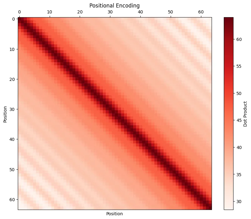
三角函数位置编码的深度解读¹中有一个章节叫远程衰减，和三角函数编码的相对性有过公式推导级别的讨论一个优良的性质：位置编码的内积值，随着相对距离的增大逐渐趋近于 $0$ ，这符合直觉：相对距离越大的输入，其位置相关性越弱。如果推导公式比较难，可以可视化三角函数位置编码的内积，得到类似confusion matrix的可视化矩阵，见下图。

可视化远程衰减矩阵：

相对和绝对位置编码

绝对位置编码

一般来说，绝对位置编码会加到输入序列中：在输入的第 $k$ 个向量 $x_k$ 中加入位置向量 $p_k$ ，即 $x_k+p_k$ ，其中 $p_k$ 只依赖于在序列的位置 $k$ 。常见的位置向量形式是三角式(Sinusoidal)和可训练式，也有其他形式²。

相对于相对位置编码，绝对位置编码的优点是计算复杂度更低。

三角函数

在Transformer文中，我们知道Sinusocidal位置编码在embed_sim后面接近于 $0$ 和 $1$ 间隔的编码，因此可以期望它有一定的外推性。

三角函数还有一个有意思的性质： $\sin(i+j)=\sin i\cos j+\cos i\sin j$ 和 $\cos(i+j)=\cos i \cos j - \sin i \sin j$ ，即位置 $i+j$ 可以表示成 $i$ 和 $j$ 的组合的形式，这提供了某种表达相对位置编码的性质。

可训练式

可训练式位置编码不去设计编码的形式，而是将编码作为可学习的参数，与输入向量相加。在视觉任务的Transformer工作中，例如DETR及其后续工作，都是位置编码都是可训练式。

不难想象，可训练式位置编码的缺点是没有外推性，即推理时无法处理超过训练时最长长度的输入序列。不过，苏神的文章⁶通过层次分解的方式，使得绝对位置编码能外推到足够的长度。

相对位置编码

相对位置并没有完整建模每个输入的位置信息，而是在计算attention的时候考虑当前位置与其他位置的相对距离，由于自然语言一般更依赖于相对位置，所以相对位置编码通常有着优秀的表现。对于相对位置编码来说，它的灵活性更大。但是，由于相对位置编码对Attention的计算进行了修改，它的计算复杂度和attention计算同样是 $O(n^2)$ ，效率上显然低于绝对位置编码。另外，还是由于修改了Attention计算，后面对Attention的优化工作就无法执行。总的来说，相对和绝对位置编码是一个trade-off，而后面将要介绍的RoPE编码是融合了相对位置和绝对位置的一种编码方式，成为LLM的标配。

考虑一般形式的相对位置编码⁴:

\begin{equation}\left\{\begin{aligned} \boldsymbol{q}_i =&\, (\boldsymbol{x}_i + \boldsymbol{p}_i)\boldsymbol{W}_Q \\ \boldsymbol{k}_j =&\, (\boldsymbol{x}_j + \boldsymbol{p}_j)\boldsymbol{W}_K \\ \boldsymbol{v}_j =&\, (\boldsymbol{x}_j + \boldsymbol{p}_j)\boldsymbol{W}_V \\ a_{i,j} =&\, softmax\left(\boldsymbol{q}_i \boldsymbol{k}_j^{\top}\right)\\ \boldsymbol{o}_i =&\, \sum_j a_{i,j}\boldsymbol{v}_j \end{aligned}\right.\end{equation}

其中 $i$ 和 $j$ 对应序列中的不同位置。

我们将 $q_i$ 和 $k_j$ 代入到 $softmax$ 的公式的 $q_i k_j^\top$ 中去，得到：

\begin{equation} \boldsymbol{q}_i \boldsymbol{k}_j^{\top} = \left(\boldsymbol{x}_i + \boldsymbol{p}_i\right)\boldsymbol{W}_Q \boldsymbol{W}_K^{\top}\left(\boldsymbol{x}_j + \boldsymbol{p}_j\right)^{\top} = \left(\boldsymbol{x}_i \boldsymbol{W}_Q + \boldsymbol{p}_i \boldsymbol{W}_Q\right)\left(\boldsymbol{W}_K^{\top}\boldsymbol{x}_j^{\top} + \boldsymbol{W}_K^{\top}\boldsymbol{p}_j^{\top}\right) \end{equation}

作为对比，假如我们没有相对位置编码的偏置，应该是：

\boldsymbol{q}_i \boldsymbol{k}_j^{\top}=\boldsymbol{x}_i \boldsymbol{W}_Q \boldsymbol{W}_K^{\top} \boldsymbol{x}_j^{\top}

那么，去掉 $\boldsymbol{p}_i \boldsymbol{W}_Q$ ，并且将 $\boldsymbol{p}_j \boldsymbol{W}_K$ 替换成 $\boldsymbol{R}_{i,j}^{K}$ :

\begin{equation} a_{i,j} = softmax\left(\boldsymbol{x}_i \boldsymbol{W}_Q\left(\boldsymbol{x}_j\boldsymbol{W}_K + \color{green}{\boldsymbol{R}_{i,j}^K}\right)^{\top}\right) \end{equation}

最后，在使用 $v_i$ 计算加权和时: $\boldsymbol{o}_i =\sum\limits_j a_{i,j}\boldsymbol{v}_j = \sum\limits_j a_{i,j}(\boldsymbol{x}_j\boldsymbol{W}_V + \boldsymbol{p}_j\boldsymbol{W}_V)$ ，将 $\boldsymbol{p}_j\boldsymbol{W}_V$ 替换成 $\boldsymbol{R}_{i,j}^{V}$ :

\begin{equation} \boldsymbol{o}_i = \sum_j a_{i,j}\left(\boldsymbol{x}_j\boldsymbol{W}_V + \color{green}{\boldsymbol{R}_{i,j}^{V}}\right) \end{equation}

那么， $\boldsymbol{R}_{i,j}^{K}$ 和 $\boldsymbol{R}_{i,j}^{V}$ 是什么？它们怎么体现出相对的位置关系的？所谓相对位置，是”将本来依赖于二元坐标 $(i,j)$ 的向量 $\boldsymbol{R}_{i,j}^{K}, \boldsymbol{R}_{i,j}^{V}$ ，改为只依赖于相对距离 $i−j$ ，并且通常来说会进行截断，以适应不同任意的距离”:

\begin{equation}\begin{aligned} \boldsymbol{R}_{i,j}^{K} = \boldsymbol{p}_K\left[\text{clip}(i-j, p_{\min}, p_{\max})\right] \\ \boldsymbol{R}_{i,j}^{V} = \boldsymbol{p}_V\left[\text{clip}(i-j, p_{\min}, p_{\max})\right] \end{aligned}\end{equation}

$\boldsymbol{p}_K$ 和 $\boldsymbol{p}_V$ 是可以是可训练式活三角函数式的，都可以达到处理任意长度文本的需求。

相对位置编码还有一些形式，例如XLNET，T5或DeBERTa，都是对上面的一般式进行了一些变化²。

旋转式位置编码

“一般来说，绝对位置编码具有实现简单、计算速度快等优点，而相对位置编码则直接地体现了相对位置信号，跟我们的直观理解吻合，实际性能往往也更好。由此可见，如果可以通过绝对位置编码的方式实现相对位置编码，那么就是集各家之所长。” 旋转式位置编码，英文是Rotary Position Embedding (RoPE) 是一种“绝对位置编码的方式实现相对位置编码”的设计³：简单说来，RoPE应用旋转矩阵在输入序列赋予绝对位置信息，通过注意力计算（内积）赋予序列相对位置信息。

复数的表示

矩阵表示

复数系 $\mathbb{C}$ 可以看作是二维平面 $\mathbb{R}^2$ （复数平面），任意复数 $z$ 可唯一的表示为 $z=a+bi$ ， $i$ 表示的是虚部， $a$ 和 $b$ 都是实数。也就是说，复数 $a+bi$ 与实数对 $(a,b)$ 组成有序对：

$a+bi \leftrightarrow (a,b)$

复数系满足加法和乘法结构： $(a+bi)+(c+di)=(a+c)+(b+d)i$ 和 $(a+bi)(c+di)=(ac-bd)+(bc+ad)i$

复数也可以用一个 $2 \times 2$ 的实矩阵表示，定义复数 $a+bi$ 到矩阵的映射 $f$ ：

f(a + bi) = \begin{bmatrix} a & -b \\ b & a \end{bmatrix}

这样定义的矩阵表示保留了复数的加法和乘法代数结构（可以将复数系 $\mathbf{C}$ 和它的矩阵表达 $\mathbf{R}^{2 \times 2}$ 是两个同态的代数结构）

加法

\begin{align*} f((a + bi) + (c + di)) &= f((a + c) + (b + d) i) \\ &= \begin{bmatrix} a + c & -b-d \\ b + d & a + c \end{bmatrix} \\ &= \begin{bmatrix} a & -b \\ b & a \end{bmatrix} + \begin{bmatrix} c & -d \\ d & c \end{bmatrix} \end{align*}

乘法

\begin{align*} f((a + bi) (c + di)) &= f((ac - bd) + (bc + ad) i) \\ &= \begin{bmatrix} ac - bd & -bc-ad \\ bc + ad & ac - bd \end{bmatrix} \\ &= \begin{bmatrix} a & -b \\ b & a \end{bmatrix} \begin{bmatrix} c & -d \\ d & c \end{bmatrix} \end{align*}

另外两个复数的矩阵表示保留的是：

复数矩阵表示的行列式与复数的模长相等，都是 $a^2+b^2$
复数的共轭(复数 $a+bi$ 的共轭是 $a-bi$ )等于复数矩阵表示的转置

为什么复数可以映射到一个 $2 \times 2$ 的矩阵表示呢？以下是deepseek的回答：

复数可以用矩阵表示的原因在于它们的代数结构同构于特定的 $2 \times 2$ 实矩阵组成的环。

复数可以看作是一个二维实向量空间，基为 $1$ 和 $i$ ，而矩阵表示可能对应于这个向量空间上的线性变换。比如，复数乘法可以视为一种线性变换，作用于二维实向量空间上，对应的矩阵就是这样的形式。考虑将复数 $a + bi$ 视为一个线性变换，它作用在另一个复数 $x + yi$ 上，即乘以 $(a + bi)$ 后的结果。这个线性变换可以用矩阵来表示。例如，复数 $a + bi$ 乘以 $x + yi$ 得到 $(ax - by) + (ay + bx)i$ 。如果我们将复数 $x + yi$ 表示为向量 $\begin{bmatrix} x \\ y \end{bmatrix}$ ，那么这个乘法对应的线性变换就是：

\begin{bmatrix} a & -b \\ b & a \end{bmatrix} \begin{bmatrix} x \\ y \end{bmatrix}= \begin{bmatrix} ax - by \\ bx + ay \end{bmatrix}

这正是上面的矩阵形式。因此，每个复数 $a + bi$ 都可以对应到这样一个线性变换矩阵，而这个矩阵的乘法对应于复数的乘法，加法对应于复数的加法。因此，复数域同构于这些矩阵构成的矩阵环的一个子环。

极坐标表示

复数 $z=a+bi$ 可以用模长和幅角表示：

z=r(\sin \theta + i\sin \theta)

其中， $r=\sqrt{a^2+b^2}$ ，幅角 $\theta=arctan(\frac{b}{a})$ 。

共轭使用极坐标表示：

\overline{z} = r(\sin \theta - i\sin \theta)

欧拉公式：

e^{i\theta}=\cos \theta + i \sin \theta

因此，复数可以进一步写成：

z = re^{i\theta}

共轭使用欧拉公式：

\overline{re^{i\theta}} = re^{-i\theta}

RoPE

因为RoPE和复数的表示紧密相关，所以先对复数的表示做了铺垫，现在进入正题“旋转位置编码”。其实，从前面的章节中可以看到，三角函数编码是一种绝对位置编码，因为它提供了每个位置的确定性的编码信息，同时它也可以提供一些隐含的相对位置信息，可以说三角函数位置编码是性质非常不错的设计。但是相对位置并没有显示的去表示，RoPE是对此的改进，它是使用“绝对位置编码的方式实现相对位置编码”³⁷。

有位置为 $m$ 的query向量 $\mathbf{q}_m$ ，以及在位置 $n$ 的key向量 $\mathbf{k}_n$ ，经过函数 $f$ 变换后，赋予绝对位置信息，并且再注意力计算(内积)中表达相对位置关系 $m-n$ 的位置信息：

对函数 $f$ 进一步说明，作为对比，在三角函数编码中， $f$ 相当于是 $f(q,m)=q+p_m$ ， $p_m$ 就是提前计算好的三角函数编码。但是并不是说，只有相加这种方式，实际上在RoPE中，是使用了矩阵乘法(复数的旋转矩阵表示)的方式。

\tilde{\boldsymbol{q}}_m = \boldsymbol{f}(\boldsymbol{q}, m), \quad\tilde{\boldsymbol{k}}_n = \boldsymbol{f}(\boldsymbol{k}, n)

\langle\boldsymbol{f}(\boldsymbol{q}, m), \boldsymbol{f}(\boldsymbol{k}, n)\rangle = g(\boldsymbol{q},\boldsymbol{k},m-n)

目的是要找到这样的函数 $f$ ，满足上面的公式。先一步一步从简单的情况看起， $\boldsymbol{q}_m$ 和 $\boldsymbol{k}_n \in \mathbb{R}^2$ 都是二维向量。作为一个不是很贴切的联想，三角位置编码的值最小的单元是一对 $\sin$ 和 $\cos$ 。

RoPE巧妙将 $f$ 定义为一个和绝对位置有关的旋转矩阵作用于输入序列：

\boldsymbol{f}(\boldsymbol{q}, m) =\begin{bmatrix}\cos m\theta & -\sin m\theta\\ \sin m\theta & \cos m\theta\end{bmatrix} \begin{bmatrix}q_0 \\ q_1\end{bmatrix}

由于一个复数既有矩阵的表示也有极坐标的表示：

\boldsymbol{f}(\boldsymbol{q}, m) = \boldsymbol{q} e^{\text{i}m\theta}

把上式带入到内积计算中，并且

\langle\boldsymbol{f}(\boldsymbol{q}, m), \boldsymbol{f}(\boldsymbol{k}, n)\rangle= \langle (\boldsymbol{q_m} e^{\text{i}m\theta}) (\boldsymbol{k_n} e^{\text{i}n\theta}) \rangle= \text{Re} \left[(\boldsymbol{q_m} e^{\text{i}m\theta}) (\boldsymbol{k_n} e^{\text{i}n\theta})^{*} \right] = \text{Re}\left[\boldsymbol{q}_m \boldsymbol{k}_n^* e^{\text{i}(m-n)\theta}\right]

你会发现：如此定义的 $f$ 在内积操作（注意力计算）时赋予了相对的位置信息！完美实现既有绝对位置又有相对位置！

把二维扩展到 $d$ 维度：

\scriptsize{\begin{bmatrix} \cos m\theta_0 & -\sin m\theta_0 & 0 & 0 & \cdots & 0 & 0 \\ \sin m\theta_0 & \cos m\theta_0 & 0 & 0 & \cdots & 0 & 0 \\ 0 & 0 & \cos m\theta_1 & -\sin m\theta_1 & \cdots & 0 & 0 \\ 0 & 0 & \sin m\theta_1 & \cos m\theta_1 & \cdots & 0 & 0 \\ \vdots & \vdots & \vdots & \vdots & \ddots & \vdots & \vdots \\ 0 & 0 & 0 & 0 & \cdots & \cos m\theta_{d/2-1} & -\sin m\theta_{d/2-1} \\ 0 & 0 & 0 & 0 & \cdots & \sin m\theta_{d/2-1} & \cos m\theta_{d/2-1} \\ \end{bmatrix} \begin{bmatrix}q_0 \\ q_1 \\ q_2 \\ q_3 \\ \vdots \\ q_{d-2} \\ q_{d-1}\end{bmatrix}}

由于矩阵过于稀疏，使用下面公式更简洁：

\begin{bmatrix}q_0 \\ q_1 \\ q_2 \\ q_3 \\ \vdots \\ q_{d-2} \\ q_{d-1} \end{bmatrix}\otimes\begin{bmatrix}\cos m\theta_0 \\ \cos m\theta_0 \\ \cos m\theta_1 \\ \cos m\theta_1 \\ \vdots \\ \cos m\theta_{d/2-1} \\ \cos m\theta_{d/2-1} \end{bmatrix} + \begin{bmatrix}-q_1 \\ q_0 \\ -q_3 \\ q_2 \\ \vdots \\ -q_{d-1} \\ q_{d-2} \end{bmatrix}\otimes\begin{bmatrix}\sin m\theta_0 \\ \sin m\theta_0 \\ \sin m\theta_1 \\ \sin m\theta_1 \\ \vdots \\ \sin m\theta_{d/2-1} \\ \sin m\theta_{d/2-1} \end{bmatrix}

其中， $\otimes$ 表示逐元素相乘， $\theta_j = 10000^{−\frac{2j}{d}}$ 与三角函数编码一致。

RoPE的实现

RoPE的代码有好几种 !

苏神在roformer有简单代码实现，和上一节最后的实现公式完全一致：

sinusoidal_pos.shape = [1, seq_len, hidden_size] # Sinusoidal position embeddings
qw.shape = [batch_size, seq_len, num_heads, hidden_size]  # query hiddens
kw.shape = [batch_size, seq_len, num_heads, hidden_size]  # key hiddens

# 这里cos是奇数部分，sin是偶数部分，但是并且重复了一次后和原hidden_size长度一致
cos_pos = repeat_elements(sinusoidal_pos[..., None, 1::2], rep=2, axis=-1)
sin_pos = repeat_elements(sinusoidal_pos[..., None, ::2], rep=2, axis=-1)
# 首先从qw中提取出奇数和偶数索引，而qw_odd/even: [batch_size, seq_len, num_heads, D//2]
# 重要的是沿着第5维度stack，这样stack后得到的shape是 [batch_size, seq_len, num_heads, 2, D//2]
qw2 = stack([-qw[..., 1::2], qw[..., ::2]], axis=4)
# reshape操作就有意思了，因为在2这个维度是奇数和偶数，reshape会原维度D，会实现交叉奇偶的效果
# 正好是上一节公式中交替变换的向量
qw2 = reshape(qw2, shape(qw))
qw = qw * cos_pos + qw2 * sin_pos

另外有人使用pytorch实现了另一个版本，主要是借助公式：

\begin{bmatrix}\cos m\theta_j & -\sin m\theta_j \\ \sin m\theta_j & \cos m\theta_j \end{bmatrix} \begin{bmatrix}q_{2j} \\ q_{2j-1}\end{bmatrix}

def apply_rotary(x, sinusoidal_pos=None):
    if sinusoidal_pos is None:
        return x
    sin, cos = sinusoidal_pos # [seq_len, hidden_dim//2]
    # x.shape [batch, seq_len, hidden_dim]
    x_even, x_odd = x[..., 0::2], x[..., 1::2]
    # [cos_nθ, -sin_nθ] [x_even]
    # [sin_nθ,  cos_nθ] [x_odd]
    # => [x_even * cos_nθ - x_odd * sin_nθ, x_even * sin_nθ + x_odd * cos_nθ]
    return torch.cat([x_even * cos - x_odd * sin, x_even * sin + x_odd * cos], dim=-1)

深入三角函数位置编码

位置编码性质

相加

相对性质

远程衰减

相对和绝对位置编码

绝对位置编码

三角函数

可训练式

相对位置编码

旋转式位置编码

复数的表示

矩阵表示

极坐标表示

RoPE

RoPE的实现

Footnotes